Object Detection Part 1
My goal in this series is to deploy a neural network capable of identifying and localizing pedestrians in an image (the combination of image classification and localization is called object detection). In the first part of the series I will do this by downloading a pretrained model and using transfer learning to fine tune it for my problem. In the second part, I will try to create and deploy a model from scratch.
Table of Contents
Overview
Motivation and Applications
My main motivation for this project was simply to gain an understanding of deep learning, a field I knew nothing about prior to this project. Furthermore, object detection problems tend to involve much deeper networks than object classification, and the concepts involved here are highly transferable across other deep learning domains.
Of course, object detection has some pretty cool applications in its own right. For example, security companies build on top of object detection models to do things like gait analysis and tracking people across multiple cameras. Self-driving cars need to be able to perform object detection to avoid hitting pedestrians and other cars. And one could imagine lots of fun home applications for object detection.
Why Transfer Learning
Practically speaking, you will almost always use transfer learning when dealing with neural network. The reason for this is twofold:
- Using a pretrained model drastically cuts down the amount of resources needed to fine tune a network. By using a pretrained model you will require fewer training samples and less computing time for a comparable level of accuracy.
- It is unlikely that you will be creating a deep learning model that is completely new. Most new models are really variations of existing models, so it makes sense to take advantage of existing work Consequently, transfer learning is one of the most important skills you can have with respect to deep learning
Background
What is a Neural Network
To understand what a neural network is, we can break the concept down into two components, structure and learning.
Structure: Although different model types can have additional components, all neural networks have an input layer, some number of hidden layers, and an output layer, as seen in the picture bellow.

The layers in turn are made up of nodes called neurons. All a neuron is is a container that holds a single number.
Breaking things down, the neurons in the input layer correspond to the data points we are analyzing. For example, if we are analyzing a picture, the input layer neurons correspond to the pixel values of that picture. Each neuron is then multiplied by some value, called a weight, and added together to produce a new value, which will become a neuron for the first hidden layer. So each neuron is the result of a different linear transformation on the previous layer. The neurons then undergo a non-linear transformation, called an activation function. For example, a common activation function is to map positive values to themselves and negative values to 0. The whole point of the activation function is to make our system capable of solving non-linear systems. This process is then repeated for each hidden layer, until we get to the output layer. The output layer represents the data we want. For example, if we have a dog classifier, the output layer would be 0 for "no dog" and 1 for "dog".
To help visualize the process outlined, you can look at this simplified neural network:
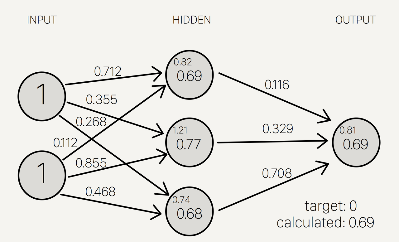
The initial neurons are (1,1) and the first transform is (0.712, 0.0112), so the initial value of the first neuron of the hidden layer is $$(1,1)*(0.712, 0.0112)= 0.712+0.0112 = 0.824 $$ That value is then placed through the activation function. In this case, the activation function is called the Sigmoid function, $S(x)= \frac{1}{e^{-x}}$ so as a final value we get: $$S(0.824) = 0.69$$ That process is then repeated for every neuron in the first layer of the model. Then to get our output layer of one neuron, we put the hidden layer (0.69, 0.77, 0.68) and apply the transform (0.116, 0.329, 0.708) to get the output value of 0.69.
Now that you know how neural networks are structured, you're probably wondering why they are structured this way, since it just looks like a lot of wheel spinning on the surface. Again, we will break this down into parts, but the main benefit of this structure is that it allows us to model complex interactions within our data. Starting from the input layer, the weights allow all of our data to interact with each other. Some weights will be higher, which means some of the input data will dominate the neuron it's mapped to, and some of the weights may even be 0, meaning that some data won't have any effect on that neuron. Therefore each neuron actually represents some interaction in the data, i.e. a neuron is a feature that we would have to specifically program in a supervised learning model. The cool thing is that each additional layer allows the features from the previous layer to interact with one another to create another feature in the next hidden layer. As a concrete example, we may input an image, and the first layer may extract distinct edges from that image, and the next layer may extract distinct shapes. Finally, the activation function serves two purposes, it allows the model to capture non-linearity, and it bounds the possible value of the neurons, which is useful for training.
Training: While there is a lot of mysticism surrounding deep learning models in pop-sci, you can really just think of neural networks as non-linear, differential optimization problems. Like any other model, you have inputs, outputs, and targets and you want the model to produce outputs as close to the targets as possible (for whatever metric of closeness you have defined). In the case of a neural network, once the structure is locked in, the only way to change the outputs is to change the value of the weights in each layer. This is done through gradient descent.
What is Transfer Learning
Transfer learning is essentially repurposing an an existing deep learning model for a new but similar task.
To understand when and why transfer learning is effective, remember that the layers in a trained model represent features that the model has learned to extract. Furthermore, the features extracted tend to become more particular to the problem as we go into deeper layers. For example, an animal classifier may have a layer that extracts basic shapes from the image, another layer that recognizes textures, and so on. As you can see from the example, the features a model learns to extract are often useful for similar tasks. So if we wanted to create a face detector, we could start from randomized layers and see which features emerged from our model. Or we could take advantage of the fact that the features extracted by our first model are useful for other image classification tasks, and use that as a starting point rather than reinvent the wheel.
A slightly more technical way of looking at transfer learning is from an optimization perspective. Remember, a neural network is composed of layers of weights that transform the data in each layer. And when we train a model, we are moving those weights to a more optimal value through gradient descent. When we use a new model, those weights' values are completely random to start. However, if we assume similar input and output, then the weights of our pretrained model are likely closer to their optimum values than completely random weights. So our pretrained model requires less adjustment (training steps) to be optimized.
We can break down transfer learning into the following steps:
- download a model that has already been trained on a dataset
- make whatever adjustments you want to test on the model (e.g. adjust the learning rate)
- strip last layers of the existing model and replace them with randomized layers
- fine-tune layers on new data
- Verify Results
Modeling
Here I will go through the steps I went through to get my model up and running, from installing tensor flow, to preparing the data, to training the model
Installing TensorFlow and Object Detection API
To start, I highly recommend creating a virtual environment either through Anaconda or Python environments to help manage version requirements. Within your environment install the necessary packages.
pip install tensorflow
pip install Cython
pip install pillow
pip install lxml
pip install jupyter
pip install matplotlib
Then to install the Object Detection API, you need to download the tensorflow models repo by running the following command on your terminal
git clone https://github.com/tensorflow/models.git
Then on the terminal CD into tensorflow/models/research/ and compile protobuf by running
# From tensorflow/models/research/
protoc object_detection/protos/*.proto --python_out=.
Finally, add the libraries to your pythonpath by running:
# From tensorflow/models/research/
export PYTHONPATH=$PYTHONPATH:`pwd`:`pwd`/slim
every time you open a new terminal window
Preparing the Data
The data I am using comes from https://www.kaggle.com/smeschke/pedestrian-dataset#crosswalk.csv. It consists of 3 videos of pedestrians using crosswalks in different situations as well as CSV files for each video which give the bounding box information for the pedestrians in the video in the following format, (x, y, height, width).
My goal in this section is to break down each video into its component frames in jpg format. I then need to create a data frame which contains the following columns: file path, width, height, class, xmin, xmax, ymin, ymax
It is also worth noting that all of the models in the object detection API are size agnostic. They perform all necessary image padding and scaling for you. However, I will go over how to do data standardization and augmentation in the next post.
Extract Images from Video
Because the data comes as video files, I will use cv2 to read it and capture frames. The code bellow carries out the following steps:
- Gets a list of videos in the data directories
- Defines a function which
- reads a video file
- creates a directory named after the video if none exists
- captures a frame and saves it as a jpeg to the directory
- applies the function to all files in the list
import cv2
import pandas as pd
import numpy as np
import os
#get list of video files
dataPath = 'data/'
dataFiles = os.listdir(dataPath)
videoFiles = [dataPath+file for file in dataFiles if file.endswith('.avi')]
#define function to turn video into images
def frame_capture(path):

    cap = cv2.VideoCapture(path)
    currentFrame = 0
    directory = path.strip('.avi')
    try:
        if not os.path.exists(directory):
            os.makedirs(directory)
    except OSError:
        print ('Error: Creating directory of data')
    # checks whether frames were extracted
    success = 1

    while success:
        # Capture frame-by-frame
        success, frame = cap.read()

        # Saves image of the current frame in jpg file
        name = directory + '/frame' + str(currentFrame) + '.jpg'
        cv2.imwrite(name, frame)

        # To stop duplicate images
        currentFrame += 1

    # When everything done, release the capture
    cap.release()
    cv2.destroyAllWindows()
#turn each video file into a directory of image files
for file in videoFiles:
    frame_capture(file)
Create CSV files for training/testing
Now that I have my images, I need to combine my image file paths with my bounding box data in the format required by the object detection API. I also need to split my data into a training set and testing set.
boundingBoxFiles = ['data/night.csv', 'data/fourway.csv', 'data/crosswalk.csv']
#Reformat CSV data into required format
pedestrian_labels = pd.DataFrame()
for file in boundingBoxFiles:
    name = file.replace('/','.').split('.')[1]
    df = pd.read_csv(file)
    new_df = pd.DataFrame()
    #create columns for new dataframe
    new_df['filename'] = df.index.astype(str)
    new_df['filename'] = 'data/'+ name+ '/frame'+ new_df['filename']+ '.jpg'
    new_df['width'] = df.w
    new_df['height'] = df.h
    new_df['class'] = 'pedestrian'
    new_df['xmin'] = df.x
    new_df['ymin'] = df.y
    new_df['xmax'] = df.x + df.w
    new_df['ymax'] = df.y + df.h
    #store to central data frame
    pedestrian_labels = pedestrian_labels.append(new_df)
#split data into training and testing set, then save file
train_labels = pedestrian_labels.sample(frac=0.8,random_state=17)
test_labels = pedestrian_labels.drop(train_labels.index)
pedestrian_labels.to_csv('data/pedestrian_labels.csv', index=False)
train_labels.to_csv('data/train_labels.csv', index=False)
test_labels.to_csv('data/test_labels.csv', index=False)
#check to make sure data is in correct format
train_labels.head()
test_labels.head()
Convert CSV to TFR Format
In order to use the models, tensorflow requires you to have your data in TFRecord format. Luckily, the object detection API has a script for converting the CSV files created in the previous step to TFR files. The script is called "generate_tfrecord.py" and it is located under the file path "TensorFlow/models/research/object_detection/legacy". But I'll include the code bellow so you can just copy and paste. I will also give a link to a video which does a good job of explaining the TFRecord format and how to use it. https://www.youtube.com/watch?v=oxrcZ9uUblI
"""
Usage:

# Create train data:
python generate_tfrecord.py --label=<LABEL> --csv_input=<PATH_TO_ANNOTATIONS_FOLDER>/train_labels.csv  --output_path=<PATH_TO_ANNOTATIONS_FOLDER>/train.record

# Create test data:
python generate_tfrecord.py --label=<LABEL> --csv_input=<PATH_TO_ANNOTATIONS_FOLDER>/test_labels.csv  --output_path=<PATH_TO_ANNOTATIONS_FOLDER>/test.record
"""

from __future__ import division
from __future__ import print_function
from __future__ import absolute_import

import os
import io
import pandas as pd
import tensorflow as tf

from PIL import Image
from object_detection.utils import dataset_util
from collections import namedtuple, OrderedDict

flags = tf.app.flags
flags.DEFINE_string('csv_input', '', 'Path to the CSV input')
flags.DEFINE_string('output_path', '', 'Path to output TFRecord')
flags.DEFINE_string('label', '', 'Name of class label')
FLAGS = flags.FLAGS


# TO-DO replace this with label map
def class_text_to_int(row_label):
    if row_label == FLAGS.label:  # 'ship':
        return 1
    else:
        None


def split(df, group):
    data = namedtuple('data', ['filename', 'object'])
    gb = df.groupby(group)
    return [data(filename, gb.get_group(x)) for filename, x in zip(gb.groups.keys(), gb.groups)]


def create_tf_example(group, path):
    with tf.gfile.GFile(os.path.join(path, '{}'.format(group.filename)), 'rb') as fid:
        encoded_jpg = fid.read()
    encoded_jpg_io = io.BytesIO(encoded_jpg)
    image = Image.open(encoded_jpg_io)
    width, height = image.size

    filename = group.filename.encode('utf8')
    image_format = b'jpg'
    xmins = []
    xmaxs = []
    ymins = []
    ymaxs = []
    classes_text = []
    classes = []

    for index, row in group.object.iterrows():
        xmins.append(row['xmin'] / width)
        xmaxs.append(row['xmax'] / width)
        ymins.append(row['ymin'] / height)
        ymaxs.append(row['ymax'] / height)
        classes_text.append(row['class'].encode('utf8'))
        classes.append(class_text_to_int(row['class']))

    tf_example = tf.train.Example(features=tf.train.Features(feature={
        'image/height': dataset_util.int64_feature(height),
        'image/width': dataset_util.int64_feature(width),
        'image/filename': dataset_util.bytes_feature(filename),
        'image/source_id': dataset_util.bytes_feature(filename),
        'image/encoded': dataset_util.bytes_feature(encoded_jpg),
        'image/format': dataset_util.bytes_feature(image_format),
        'image/object/bbox/xmin': dataset_util.float_list_feature(xmins),
        'image/object/bbox/xmax': dataset_util.float_list_feature(xmaxs),
        'image/object/bbox/ymin': dataset_util.float_list_feature(ymins),
        'image/object/bbox/ymax': dataset_util.float_list_feature(ymaxs),
        'image/object/class/text': dataset_util.bytes_list_feature(classes_text),
        'image/object/class/label': dataset_util.int64_list_feature(classes),
    }))
    return tf_example


def main(_):
    writer = tf.python_io.TFRecordWriter(FLAGS.output_path)
    path = os.path.join(os.getcwd(), '')
    examples = pd.read_csv(FLAGS.csv_input)
    grouped = split(examples, 'filename')
    for group in grouped:
        tf_example = create_tf_example(group, path)
        writer.write(tf_example.SerializeToString())

    writer.close()
    output_path = os.path.join(os.getcwd(), FLAGS.output_path)
    print('Successfully created the TFRecords: {}'.format(output_path))


if __name__ == '__main__':
    tf.app.run()
Once you have the above code in your working directory named as generate_tfrecord.py, you can convert the csv files by running the following code:
python generate_tfrecord.py --label=pedestrian --csv_input=data/train_labels.csv --output_path=data/train.record
python generate_tfrecord.py --label=pedestrian --csv_input=data/test_labels.csv --output_path=data/test.record
You just have to adjust the file paths that contain your training and testing data
Prepare the Model
Now that the data is in TFRrecords format, we are ready to download a model for transfer learning. First, we will need to choose a model to download. There is a list of models here which you can download, and which contain a model checkpoint and configuration file. I chose to use SSD mobilenet v1 because speed seemed more important for working with video. Once you download the model, you will need to change the configuration file. Specifically, you will need to change the number of classes, make sure the feature extractor type is set to the model you've downloaded, and then change the input paths. You can find these by searching for "PATH_TO_BE_CONFIGURED" in the file. One of the paths you need to configure is called "label_map_path". This is a file that you need to create, and it is just a mapping of the class labels in your training data to an integer. I am attaching a copy of my configuration file as well as my map for reference. I also reduced the batch size in my config file as well as the number of training steps, since I was doing the training on my personal laptop.
#Label map saved as label_map.pbtxt
item{
  id:1
  name:'pedestrian'
}
#Config file

# SSD with Mobilenet v1, configured for Oxford-IIIT Pets Dataset.
# Users should configure the fine_tune_checkpoint field in the train config as
# well as the label_map_path and input_path fields in the train_input_reader and
# eval_input_reader. Search for "PATH_TO_BE_CONFIGURED" to find the fields that
# should be configured.

model {
  ssd {
    num_classes: 1
    box_coder {
      faster_rcnn_box_coder {
        y_scale: 10.0
        x_scale: 10.0
        height_scale: 5.0
        width_scale: 5.0
      }
    }
    matcher {
      argmax_matcher {
        matched_threshold: 0.5
        unmatched_threshold: 0.5
        ignore_thresholds: false
        negatives_lower_than_unmatched: true
        force_match_for_each_row: true
      }
    }
    similarity_calculator {
      iou_similarity {
      }
    }
    anchor_generator {
      ssd_anchor_generator {
        num_layers: 6
        min_scale: 0.2
        max_scale: 0.95
        aspect_ratios: 1.0
        aspect_ratios: 2.0
        aspect_ratios: 0.5
        aspect_ratios: 3.0
        aspect_ratios: 0.3333
      }
    }
    image_resizer {
      fixed_shape_resizer {
        height: 300
        width: 300
      }
    }
    box_predictor {
      convolutional_box_predictor {
        min_depth: 0
        max_depth: 0
        num_layers_before_predictor: 0
        use_dropout: false
        dropout_keep_probability: 0.8
        kernel_size: 1
        box_code_size: 4
        apply_sigmoid_to_scores: false
        conv_hyperparams {
          activation: RELU_6,
          regularizer {
            l2_regularizer {
              weight: 0.00004
            }
          }
          initializer {
            truncated_normal_initializer {
              stddev: 0.03
              mean: 0.0
            }
          }
          batch_norm {
            train: true,
            scale: true,
            center: true,
            decay: 0.9997,
            epsilon: 0.001,
          }
        }
      }
    }
    feature_extractor {
      type: 'ssd_mobilenet_v1'
      min_depth: 16
      depth_multiplier: 1.0
      conv_hyperparams {
        activation: RELU_6,
        regularizer {
          l2_regularizer {
            weight: 0.00004
          }
        }
        initializer {
          truncated_normal_initializer {
            stddev: 0.03
            mean: 0.0
          }
        }
        batch_norm {
          train: true,
          scale: true,
          center: true,
          decay: 0.9997,
          epsilon: 0.001,
        }
      }
    }
    loss {
      classification_loss {
        weighted_sigmoid {
        }
      }
      localization_loss {
        weighted_smooth_l1 {
        }
      }
      hard_example_miner {
        num_hard_examples: 3000
        iou_threshold: 0.99
        loss_type: CLASSIFICATION
        max_negatives_per_positive: 3
        min_negatives_per_image: 0
      }
      classification_weight: 1.0
      localization_weight: 1.0
    }
    normalize_loss_by_num_matches: true
    post_processing {
      batch_non_max_suppression {
        score_threshold: 1e-8
        iou_threshold: 0.6
        max_detections_per_class: 100
        max_total_detections: 100
      }
      score_converter: SIGMOID
    }
  }
}

train_config: {
  batch_size: 24
  optimizer {
    rms_prop_optimizer: {
      learning_rate: {
        exponential_decay_learning_rate {
          initial_learning_rate: 0.004
          decay_steps: 800720
          decay_factor: 0.95
        }
      }
      momentum_optimizer_value: 0.9
      decay: 0.9
      epsilon: 1.0
    }
  }
  fine_tune_checkpoint: "ssd_mobilenet_v1_coco_11_06_2017/model.ckpt"
  from_detection_checkpoint: true
  load_all_detection_checkpoint_vars: true
  # Note: The below line limits the training process to 200K steps, which we
  # empirically found to be sufficient enough to train the pets dataset. This
  # effectively bypasses the learning rate schedule (the learning rate will
  # never decay). Remove the below line to train indefinitely.
  num_steps: 50000
  data_augmentation_options {
    random_horizontal_flip {
    }
  }
  data_augmentation_options {
    ssd_random_crop {
    }
  }
}

train_input_reader: {
  tf_record_input_reader {
    input_path: "data/train.record"
  }
  label_map_path: "training/label_map.pbtxt"
}

eval_config: {
  metrics_set: "coco_detection_metrics"
  num_examples: 1100
}

eval_input_reader: {
  tf_record_input_reader {
    input_path: "data/test.record"
  }
  label_map_path: "training/label_map.pbtxt"
  shuffle: false
  num_readers: 1
}
My file configuration
This shouldn't matter that much, but I thought I should outline how my files are organized, since I've frequently referenced fill paths.
Within the TensorFlow directory I downloaded that contains the object detection API I created a workspace directory, and within that I have a directory with the following structure:
- Workspace
- Pedestrian_Project
- Data
- All of my training and testing data
- Training
- label_map.pbtxt
- ssd_mobilenet_v1_pets.config
- generate_tfrecord.py
- train.py
- ssd_mobilenet_v1_coco_11_06_2017
- Data
- Pedestrian_Project
Train the Model
Finally, to train the model, there is a script called train.py under the file path TensorFlow/models/research/object_detection/legacy/train.py. You should make a copy of the script in your working directory, and run the following command in the terminal (accommodating for your file structure).
python train.py --logtostderr --train_dir=training/ --pipeline_config_path=training/ssd_mobilenet_v1_pets.config
Assuming you have no errors, you can check training progress by running
tensorboard --logdir='training'
Which will allow you to visualize the total loss graph

Once the model is done training, you can export the inference graph. To do this, locate the script "export_inference_graph.py" located under 'TensorFlow/models/research/object_detection/export_inference_graph.py' and copy it to your working directory. Take note of the largest model checkpoint number in your training directory, as you will use it as the argument to --trained_checkpoint_prefix. In my case, it is model.ckpt-5036. You should also create an outout directory to export the trained inference graph to labeled trained-inference-graphs. Then run the following command:
python export_inference_graph.py --input_type image_tensor --pipeline_config_path training/ssd_mobilenet_v1_pets.config --trained_checkpoint_prefix training/model.ckpt-5036 --output_directory trained-inference-graphs/output_inference_graph_v1.pb
Test the Model
Once you are satisfied with your model's performance, we can test the model. To do this, I copied the utils folder from the object detection folder, and ran the following code. While
import numpy as np
import os
import six.moves.urllib as urllib
import sys
import tarfile
import tensorflow as tf
import zipfile

from distutils.version import StrictVersion
from collections import defaultdict
from io import StringIO
import matplotlib
from matplotlib import pyplot as plt
from PIL import Image

# This is needed since the notebook is stored in the object_detection folder.
sys.path.append("..")
from object_detection.utils import ops as utils_ops

if StrictVersion(tf.__version__) < StrictVersion('1.9.0'):
  raise ImportError('Please upgrade your TensorFlow installation to v1.9.* or later!')
# This is needed to display the images.
matplotlib.use('TkAgg')
%matplotlib inline
from utils import label_map_util

from utils import visualization_utils as vis_util
# What model to download.
MODEL_NAME = 'output_inference_graph_v1.pb'

# Path to frozen detection graph. This is the actual model that is used for the object detection.
PATH_TO_FROZEN_GRAPH = MODEL_NAME + '/frozen_inference_graph.pb'

# List of the strings that is used to add correct label for each box.
PATH_TO_LABELS = os.path.join('training', 'label_map.pbtxt')

NUM_CLASSES = 1
detection_graph = tf.Graph()
with detection_graph.as_default():
  od_graph_def = tf.GraphDef()
  with tf.gfile.GFile(PATH_TO_FROZEN_GRAPH, 'rb') as fid:
    serialized_graph = fid.read()
    od_graph_def.ParseFromString(serialized_graph)
    tf.import_graph_def(od_graph_def, name='')
category_index = label_map_util.create_category_index_from_labelmap(PATH_TO_LABELS, use_display_name=True)
def load_image_into_numpy_array(image):
  (im_width, im_height) = image.size
  return np.array(image.getdata()).reshape(
      (im_height, im_width, 3)).astype(np.uint8)
# For the sake of simplicity we will use only 2 images:
# image1.jpg
# image2.jpg
# If you want to test the code with your images, just add path to the images to the TEST_IMAGE_PATHS.
PATH_TO_TEST_IMAGES_DIR = 'test_images'
TEST_IMAGE_PATHS = [ os.path.join(PATH_TO_TEST_IMAGES_DIR, 'image{}.jpg'.format(i)) for i in range(1, 4) ]

# Size, in inches, of the output images.
IMAGE_SIZE = (12, 16)
def run_inference_for_single_image(image, graph):
  with graph.as_default():
    with tf.Session() as sess:
      # Get handles to input and output tensors
      ops = tf.get_default_graph().get_operations()
      all_tensor_names = {output.name for op in ops for output in op.outputs}
      tensor_dict = {}
      for key in [
          'num_detections', 'detection_boxes', 'detection_scores',
          'detection_classes', 'detection_masks'
      ]:
        tensor_name = key + ':0'
        if tensor_name in all_tensor_names:
          tensor_dict[key] = tf.get_default_graph().get_tensor_by_name(
              tensor_name)
      if 'detection_masks' in tensor_dict:
        # The following processing is only for single image
        detection_boxes = tf.squeeze(tensor_dict['detection_boxes'], [0])
        detection_masks = tf.squeeze(tensor_dict['detection_masks'], [0])
        # Reframe is required to translate mask from box coordinates to image coordinates and fit the image size.
        real_num_detection = tf.cast(tensor_dict['num_detections'][0], tf.int32)
        detection_boxes = tf.slice(detection_boxes, [0, 0], [real_num_detection, -1])
        detection_masks = tf.slice(detection_masks, [0, 0, 0], [real_num_detection, -1, -1])
        detection_masks_reframed = utils_ops.reframe_box_masks_to_image_masks(
            detection_masks, detection_boxes, image.shape[0], image.shape[1])
        detection_masks_reframed = tf.cast(
            tf.greater(detection_masks_reframed, 0.5), tf.uint8)
        # Follow the convention by adding back the batch dimension
        tensor_dict['detection_masks'] = tf.expand_dims(
            detection_masks_reframed, 0)
      image_tensor = tf.get_default_graph().get_tensor_by_name('image_tensor:0')
      # Run inference
      output_dict = sess.run(tensor_dict,
                             feed_dict={image_tensor: np.expand_dims(image, 0)})
      # all outputs are float32 numpy arrays, so convert types as appropriate
      output_dict['num_detections'] = int(output_dict['num_detections'][0])
      output_dict['detection_classes'] = output_dict[
          'detection_classes'][0].astype(np.uint8)
      output_dict['detection_boxes'] = output_dict['detection_boxes'][0]
      output_dict['detection_scores'] = output_dict['detection_scores'][0]
      if 'detection_masks' in output_dict:
        output_dict['detection_masks'] = output_dict['detection_masks'][0]
  return output_dict
for image_path in TEST_IMAGE_PATHS:
  image = Image.open(image_path)
  # the array based representation of the image will be used later in order to prepare the
  # result image with boxes and labels on it.
  image_np = load_image_into_numpy_array(image)
  # Expand dimensions since the model expects images to have shape: [1, None, None, 3]
  image_np_expanded = np.expand_dims(image_np, axis=0)
  # Actual detection.
  output_dict = run_inference_for_single_image(image_np, detection_graph)
  # Visualization of the results of a detection.
  vis_util.visualize_boxes_and_labels_on_image_array(
      image_np,
      output_dict['detection_boxes'],
      output_dict['detection_classes'],
      output_dict['detection_scores'],
      category_index,
      instance_masks=output_dict.get('detection_masks'),
      use_normalized_coordinates=True,
      line_thickness=8)
  plt.figure(figsize=IMAGE_SIZE)
  plt.imshow(image_np)


